Magnetic field of a solenoid

As you can see, I’m not posting much on the blog these days, but every once in a while I figure out something that I want to write down so that I can refer my students to it, and this seems like the place to do it. Like a couple of previous posts, this one comes out of the electricity and magnetism course that I teach from time to time.

In his excellent textbook Introduction to Electrodynamics, David Griffiths works out the magnetic field of an infinite solenoid as an example of the application of Ampère’s Law. He shows that the field outside the solenoid is uniform, and then he says it must be zero, because “it certainly approaches zero as you go very far away.” That word “certainly” seems to be hiding something: how do we know that the field goes to zero far away? After all, we’re talking about an infinite solenoid, in which the current keeps going forever. Is it really obvious that the field goes to zero?

(For comparison, think about the electric field caused by an infinite plane of charge. You could imagine saying that that “certainly” goes to zero as you get very far away, but it doesn’t.)

Griffiths’s arguments are usually constructed very carefully, but this is an uncharacteristic lapse. While many students will cheerfully take him at his word, some (particularly the strongest students) will want an argument to justify this conclusion. So here is one. (It’s essentially the same as the one in this document by C.E. Mungan, but I flatter myself that my explanation is a bit easier to follow.)

The argument must be based on the Biot-Savart Law, not Ampère’s Law. The reason is that you can always add a constant vector to the magnetic field in a solution to Ampère’s Law and get another solution. So Ampère’s Law alone can never convince us that the field outside is zero. In some situations like this, you can combine it with a symmetry principle to get around this, but if there is one here I can’t see it. So Biot-Savart it is.

The Biot-Savart Law tells you how to get the magnetic field caused by a given current distribution by adding up (integrating) the contributions from all of the infinitesimal current elements. I want to show that the contributions from certain current elements cancel when you’re calculating the field at a point outside the solenoid. That is, I intend to show that B = 0 everywhere outside the solenoid, not just that it goes to zero far away.

Here’s the key picture.

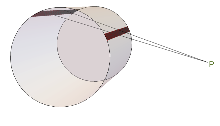
The cylinder is the solenoid. We’re trying to figure out the magnetic field at the point P. The two red bands are two thin strips of the solenoid that subtend the same small angle. I want to show that the contributions to the magnetic field at P  from those two strips cancel. Since the whole solenoid can be broken up into pairs of strips like these, that’ll show that B = 0 outside the solenoid.

Here’s the same setup, but showing just a cross section.

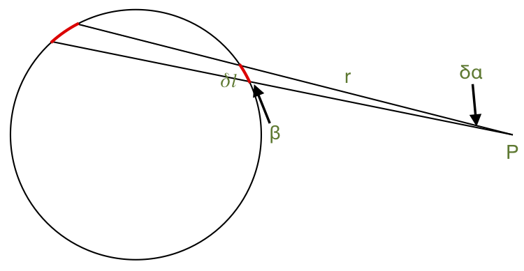
I labeled a couple of angles and lengths in this picture. They apply to the triangle formed by the point P and the closer of the two strips of current.

Here’s the main point:

The contribution to the magnetic field at P due to that strip of current is proportional to δl sin β / r. It points into the screen, straight away from you (assuming the current flows counterclockwise).

You can show that this is true by actually doing the Biot-Savart integral for this strip. The result, unless I’ve made a mistake, is

where n is the number of turns per unit length and I is the current.

But you might be able to convince yourself of it without doing the integral. The sin β comes from the cross product in the Biot-Savart law. The amount of current on that strip is proportional to its width δl. The 1/has to be there on dimensional grounds: B has to be inversely proportional to a distance, and r is the only relevant distance.

The Law of Sines tells us that sin β / r = sin δα / δl, so the magnetic field due to this strip is proportional to sin δα (and none of the other quantities in the diagram). To be specific,

(By the way, since δα is small, it’d be fine to write just δα instead of sin δα.)

Now draw the analogous triangle and do the same thing for the other of the two strips. The answer is exactly the same, except that by the right-hand rule it points the other way. So the two contributions cancel.

By the way, this argument never assumed that the solenoid was a circular cylinder. Its cross section can be any crazy shape, and you’ll always be able to chop it up into pairs of thin strips that cancel in this way.

Recordings of my grandmother

Almost 100 years ago, the folklorist Frank Clyde Brown made wax-cylinder recordings of examples of North Carolina folk music. Among these recordings are six songs sung by my grandmother Aura Holton (later Aura Godard). The recordings are part of the Duke University library collection. My brother Andy created this video containing the recordings and some background information.

The sound quality on these recordings is terrible, mostly because they’re century-old wax-cylinder recordings, but also because Brown had the habit of shaving down and reusing his wax cylinders. (The incredibly helpful librarians at Duke pointed me to an exchange of letters between Brown and a fellow folklorist who decried this practice.) As someone who likes to play around with data, I thought I’d see if I could clean them up a little.

Here’s the unfiltered original of one of the songs:

Here are five attempts I made to clean this up. I’ll tell you what I did if you’re dying to know, but for the moment I have my reasons for not going into that.


Version 1:


Version 2:


Version 3:


Version 4:


Version 5:


I’d love to know which of these sounds best (or rather, least bad — they’re all terrible!). If you have an opinion, please let me know at this survey.

(Annoyingly, UR’s WordPress configuration doesn’t seem to allow me to embed a survey in this post. It also wouldn’t let me upload WAV files, so these are all MP3s. I don’t think that the MP3 compression made much difference to the sound quality.)


2024 is right around the corner

and that means another total eclipse in North America.

For the last one, in 2017, I overlaid the path of totality on data showing the average cloud cover at the time of year of the eclipse. Here’s the same thing for the eclipse that’s coming on 8 April 2024:

And here’s a graph of the cloud cover along the part of the path that lies within the US:

I used the same data sets and followed the same procedures as last time. (The only reason the styles of the pictures are different is that I switched programming languages in the intervening years.) The graph shows the states that the path of totality goes through, although as in 2017 I left off a couple of states (and provinces) that the path just barely touches.

Last time, the cloud data varied dramatically, which is why I went to Oregon to see the eclipse. This time, there’s much less variation, at least within the US. Mexico looks quite a bit better.

I haven’t figured out what I want to do yet. Last time, my brother was supposed to join me, but he couldn’t make it. I’ll see if I can get him this time.

Pinholes and eclipses

My friend Julie Laskaris showed me a picture of sunlight passing through leaves during a partial solar eclipse, something like this:

(Image from here.)

I remember seeing the same phenomenon during an eclipse I saw in Berkeley in 1991.

The crescent shapes occur because each little gap in the leaves acts like a pinhole camera, projecting an upside-down image of the partially-blocked Sun. If you’re going to see the eclipse in a couple of weeks, look out for this effect. You can even produce it for yourself by holding up your hands so that your fingers make small gaps that the sunlight can pass through.

I was looking around for explanations of this phenomenon, and I came across this NASA page. One thing I was very interested to learn from this page is that Aristotle noted this phenomenon:

In the fourth century BC, Aristotle was puzzled. “Why is it that when the sun passes through quadrilaterals, as for instance in wickerwork, it does not produce a figure rectangular in shape but circular?” he wrote. “Why is it that an eclipse of the sun, if one looks at it through a sieve or through leaves, such as a plane-tree or other broadleaved tree, or if one joins the fingers of one hand over the fingers of the other, the rays are crescent-shaped where they reach the earth?

I’ve read a lot of Aristotle’s writing on astronomical topics, and I’ve even inflicted him on my students from time to time, but I’d never encountered this. It turns out that it’s in the book Problems, which I’d never heard of and which some people seem to think might not be Aristotle at all.

Julie is a classicist, so it was quite fitting that her showing me this picture led me to learn something about Aristotle.

Math puzzles

My brother sent me a picture of a book that one of my nephews was planning to bring with him on a long plane flight:

503856505

I was thrilled to see this, because Martin Gardner’s books are a huge reason that I am the way I am today. I suspect that lots of math and science nerds would say the same. I love the idea of yet another generation being exposed to them.

In honor of Martin Gardner, here’s a math puzzle I just saw. It was posted on the wall of the UR math department. One of the faculty there posts weekly puzzles and gives a cookie to anyone who solves them. I don’t know if this one is still up there, but if it is, and you hurry, a cookie could be yours.

A mole is on a small island at the exact center of a circular lake. A fox is at the edge of the lake. The fox wants to catch and eat the mole; the mole wants to avoid this. The mole can swim at a steady speed. The fox can’t swim but can run around the edge of the lake, four times as fast as the mole can swim. If the mole makes it to the edge of the lake, she can very quickly burrow into the ground. Can the mole escape? (That is, can she reach a point on the edge of the lake before the fox gets to that same point?)

You can assume that the fox and mole can see each other at all times, and that they can change their speed and direction instantaneously.

This is a great Gardner-esque puzzle, because you don’t need any advanced mathematics to solve it. All you need is distance = rate x time and the rule for the circumference of a circle.

If you want something harder, you can try to figure out the minimum speed that the fox must have in order to be able to catch the mole. (That is, what would you have to change the number four to, in order to change the answer?) I think I’ve worked that one out, although I could have made a mistake.

The Neyman-Scott paradox

I’m mostly posting this to let you know about Peter Coles’s nice exposition of something called the Neyman-Scott paradox. If you like thinking about probability and statistics, and in particular about the difference between Bayesian and frequentist ways of looking at things (and who doesn’t like that?), you should read it.

You should read the comments too, which have some actual defenders of the frequentist point of view. Personally, I’m terrible at characterizing frequentist arguments, because I don’t understand how those people think. To be honest, I think that Peter is a bit unfair to the frequentists, for reasons that you’ll see if you read my comment on his post. Briefly, he seems to suggest that “the frequentist approach” to this problem is not what actual frequentists would do.

The Neyman-Scott paradox is a somewhat artificial problem, although Peter argues that it’s not as artificial as some people seem to think. But the essential features of it are contained in a very common situation, familiar to anyone who’s studied statistics, namely estimating the variance of a set of random numbers.

Suppose that you have a set of measurements x1, …, xm. They’re all drawn from the same probability distribution, which has an unknown mean and variance. Your job is to estimate the mean and variance.

The standard procedure for doing this is worked out in statistics textbooks all over the place. You estimate the mean simply by averaging together all the measurements, and then you estimate the variance as

variance

That is, you add up the squared deviations from the (estimated) mean, and divide by – 1.

If nobody had taught you otherwise, you might be inclined to divide by m instead of – 1. After all, the variance is supposed to be the mean of the squared deviations. But dividing by m leads to a biased estimate: on average, it’s a bit too small. Dividing by – 1 gives an unbiased estimate.

In my experience, if a scientist knows one fact about statistics, it’s this: divide by – 1 to get the variance.

Suppose that you know that the numbers are normally distributed (a.k.a. Gaussian). Then you can find the maximum-likelihood estimator of the mean and variance. Maximum-likelihood estimators are often (but not always) used in traditional (“frequentist”) statistics, so this seems like it might be a sensible thing to do. But in this case, the maximum-likelihood estimator turns out to be that bad, biased one, with m instead of m – 1 in the denominator.

The Neyman-Scott paradox just takes that observation and presents it in very strong terms. First, they set m = 2, so that the difference between the two estimators will be most dramatic. Then they imagine many repetitions of the experiment (that is, many pairs of data points, with different means but the same variance). Often, when you repeat an experiment many times, you expect the errors to get smaller, but in this case, because the error in question is bias rather than noise (that is, because it shifts the answer consistently one way), repeating the experiment doesn’t help. So you end up in a situation where you might have expected the maximum-likelihood estimate to be good, but it’s terrible.

Bayesian methods give a thoroughly sensible answer. Peter shows that in detail for the Neyman-Scott case. You can work it out for other cases if you really want to. Of course the Bayesian calculation has to give sensible results, because the set of techniques known as “Bayesian methods” really consist of nothing more than consistently applying the rules of probability theory.

As I’ve suggested, it’s unfair to say that frequentist methods are bad because the maximum-likelihood estimator is bad. Frequentists know that the maximum-likelihood estimator doesn’t always do what they want, and they don’t use it in cases like this. In this case, a frequentist would choose a different estimator. The problem is in the word “choose”: the decision of what estimator to use can seem mysterious and arbitrary, at least to me. Sometimes there’s a clear best choice, and sometimes there isn’t. Bayesian methods, on the other hand, don’t require a choice of estimator. You use the information at your disposal to work out the probability distribution for whatever you’re interested in, and that’s the answer.

(Yes, “the information at your disposal” includes the dreaded prior. Frequentists point that out as if it were a crushing argument against the Bayesian approach, but it’s actually a feature, not a bug.)

Ranking the election forecasters

In Slate, Jordan Ellenberg asks How will we know if Nate Silver was right?

It’s a good question. If you have a bunch of models that make probabilistic predictions, is there any way to tell which one was right? Every model will predict some probability for the outcome that actually occurs. As long as that probability is nonzero, how can you say the model was wrong?

Essentially every question that a scientist asks is of this form. Because measurements always have some uncertainty, you can virtually never say that the probability of any given outcome is exactly zero, so how can you ever rule anything out?

The answer, of course, is statistics. You don’t rule things out with absolute certainty, but you rule them out with high confidence if they fit the data badly. And “fit the data badly” essentially means “have a low probability of occurring.”

So Ellenberg proposes that all the modelers publish detailed probabilities for all possible outcomes (specifically, all possible combinations of victories by the candidates in each state). Once we know the outcome, the one who assigned the highest probability to it is the best.

In statistics terminology, what he’s proposing is simply ranking the models by likelihood. That is indeed a standard thing to do, and if I had to come up with something, it’s what I’d suggest too. In this case, though, it’s probably not going to give a definitive answer, simply because all the forecasters will probably have comparable probabilities for the one outcome that will occur.

All of those probabilities will be low, because there are lots of possible outcomes, and any given one is unlikely. That doesn’t matter. What matters is whether they’re all similar. If 538 predicts a probability of 0.8%, and Princeton Election Consortium predicts 0.0000005%, then I agree that 538 wins. But what if the two predictions are 0.8% and 0.5%? The larger number still wins, but how strong is that evidence?

The way to answer that question is to use a technique called reasoning (or as some old-fashioned people insist on calling it, Bayesian reasoning). Bayes’s theorem gives a way of turning those likelihoods into posterior probabilities, which are the probabilities that any given model is correct, given the evidence. The answer depends on the prior probabilities — how likely you thought each model was before the data came in. If, as I suspect, the likelihoods come out comparable to each other, then the final outcome depends strongly on the prior probabilities. That is, the new information won’t change your mind all that much.

If things turn out that way, then Ellenberg’s proposal won’t answer the question, but that’s because there won’t be any good way to answer the question. The Bayesian analysis is the correct one, and if it says that the posterior distribution depends strongly on the prior, then that means that the available data don’t tell you who’s better, and there’s nothing you can do about it.


Gerrymandering without gerrymanderers

The Washington Post has a nice graphic explaining how gerrymandering works.

imrs

If the people drawing the district lines prefer one party, they can draw the lines as on the right: they pack as many opponents as possible into a few districts, so that those opponents win those districts in huge landslides. Then they spread out their people to win the other districts by slight majorities.

The solution people generally propose is to put the district-drawing power into the hands of non-partisan people or groups. While I think this is certainly a good idea, it’s worth mentioning that you can get “unfair” results even without deliberate gerrymandering. In particular, if members of the political parties happen to cluster in different ways, then even a nonpartisan system of drawing districts can lead to one party being overrepresented.

I don’t propose to dig into the details of this as it affects US politics. Briefly, the US House of Representatives is more Republican than it “should” be: the fraction of representatives who are Republican is more than the nationwide fraction of votes for republicans in House races. Similar statements are true for various states’ US House delegations and for state legislatures, sometimes favoring the Democrats. No doubt you can find a lot more about this if you dig around a bit. Instead, I just want to illustrate with a made-up example how you can get gerrymandering-like results even if no one is deliberately gerrymandering.

To forestall any misunderstanding, let me be 100% clear: I am not saying that there is no deliberate gerrymandering in US politics. I am saying that it need not be the whole explanation, and that even if we implemented a nonpartisan redistricting system, some disparity could remain.

I should also add that nothing I’m going to say is original to me. On the contrary, people who think about this stuff have known about it forever. But a lot of my politically-aware friends, who know all about deliberate gerrymandering, haven’t thought about the ways that “automatic gerrymandering” can happen.

Imagine a country called Squareland, whose population is distributed evenly throughout a square area. Half the population are Whigs, and half are Mugwumps. As it happens, the two political parties are unevenly distributed, with more Whigs in some areas and more Mugwumps in others:
popdist1new
The bluer a region is, the more Whigs live there. But remember, each region has the same total number of people, and the total number of Whigs and Mugwumps nationwide are the same.

You ask a nonpartisan group to divide this region up into 400 Congressional districts. They’re not trying to help one party or another, so they decide to go for simple, compact districts:

popdist1gridnew

Each district has an election and comes out either Whig or Mugwump, depending on who has a majority in the local population. In this particular example, you get 197 Mugwumps and 203 Whigs. pretty good.

Now suppose that the people are distributed differently:

popdist2new

Note that the blue regions are much more compact. There’s lots of dull red area, which is majority-Mugwump, but no bright red extreme Mugwump majorities. The blue regions, on the other hand, are extreme. The result is that there’s a lot more red area than blue, even though there are equal numbers of red folks and blue folks.

Use the same districts:

popdist2gridnew

This time, the Mugwumps win 245 seats, and the Whigs get only 155. Nobody deliberately drew district lines to disenfranchise the Whigs, but it happened anyway. And the reason it happened is very similar to what you’d get with deliberate gerrymandering: the Whigs got concentrated into a small number of districts with big majorities.

Once again, I’m not saying that this is what’s happened in the US House of Representatives. On the contrary, the evidence of deliberate gerrymandering is very strong, and given the incentives, it would be quite surprising if it did not occur. But if members of one party tend to “clump” more strongly than members of the other party, then this sort of effect can certainly occur, and could form a part of the discrepancy we see.


UR is a place “Where Great Research Meets Great Teaching”

According to the Wall Street Journal (paywall, unfortunately).

Screenshot 2016-10-07 14.12.51Most of the various college rankings strike me as somewhat silly, but I’ll make an exception for this one, because it says something nice about my home institution, which coincides very well with my own impression. Lots of places claim to be good at both teaching and research, but my experience at UR is that we really mean it. The faculty are excited both about their scholarship and about working closely with undergraduates, and the university’s reward structure conveys that both are valued.

I always say that student-faculty research is the best thing about this place.  I’m glad the WSJ agrees.

In case you’re wondering, the data used to generate this list consisted of two pieces: number of research papers per faculty member, and a student survey asking about faculty accessibility and opportunities for collaborative learning. A school had to do well on both to make the list, although I don’t think they said exact recipe for combining them.