Month: November 2016

I’m mostly posting this to let you know about Peter Coles’s nice exposition of something called the Neyman-Scott paradox. If you like thinking about probability and statistics, and in particular about the difference between Bayesian and frequentist ways of looking at things (and who doesn’t like that?), you should read it.

You should read the comments too, which have some actual defenders of the frequentist point of view. Personally, I’m terrible at characterizing frequentist arguments, because I don’t understand how those people think. To be honest, I think that Peter is a bit unfair to the frequentists, for reasons that you’ll see if you read my comment on his post. Briefly, he seems to suggest that “the frequentist approach” to this problem is not what actual frequentists would do.

The Neyman-Scott paradox is a somewhat artificial problem, although Peter argues that it’s not as artificial as some people seem to think. But the essential features of it are contained in a very common situation, familiar to anyone who’s studied statistics, namely estimating the variance of a set of random numbers.

Suppose that you have a set of measurements x₁, …, x_m. They’re all drawn from the same probability distribution, which has an unknown mean and variance. Your job is to estimate the mean and variance.

The standard procedure for doing this is worked out in statistics textbooks all over the place. You estimate the mean simply by averaging together all the measurements, and then you estimate the variance as

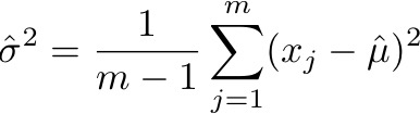
That is, you add up the squared deviations from the (estimated) mean, and divide by m – 1.

If nobody had taught you otherwise, you might be inclined to divide by m instead of m – 1. After all, the variance is supposed to be the mean of the squared deviations. But dividing by m leads to a biased estimate: on average, it’s a bit too small. Dividing by m – 1 gives an unbiased estimate.

In my experience, if a scientist knows one fact about statistics, it’s this: divide by m – 1 to get the variance.

Suppose that you know that the numbers are normally distributed (a.k.a. Gaussian). Then you can find the maximum-likelihood estimator of the mean and variance. Maximum-likelihood estimators are often (but not always) used in traditional (“frequentist”) statistics, so this seems like it might be a sensible thing to do. But in this case, the maximum-likelihood estimator turns out to be that bad, biased one, with m instead of m – 1 in the denominator.

The Neyman-Scott paradox just takes that observation and presents it in very strong terms. First, they set m = 2, so that the difference between the two estimators will be most dramatic. Then they imagine many repetitions of the experiment (that is, many pairs of data points, with different means but the same variance). Often, when you repeat an experiment many times, you expect the errors to get smaller, but in this case, because the error in question is bias rather than noise (that is, because it shifts the answer consistently one way), repeating the experiment doesn’t help. So you end up in a situation where you might have expected the maximum-likelihood estimate to be good, but it’s terrible.

Bayesian methods give a thoroughly sensible answer. Peter shows that in detail for the Neyman-Scott case. You can work it out for other cases if you really want to. Of course the Bayesian calculation has to give sensible results, because the set of techniques known as “Bayesian methods” really consist of nothing more than consistently applying the rules of probability theory.

As I’ve suggested, it’s unfair to say that frequentist methods are bad because the maximum-likelihood estimator is bad. Frequentists know that the maximum-likelihood estimator doesn’t always do what they want, and they don’t use it in cases like this. In this case, a frequentist would choose a different estimator. The problem is in the word “choose”: the decision of what estimator to use can seem mysterious and arbitrary, at least to me. Sometimes there’s a clear best choice, and sometimes there isn’t. Bayesian methods, on the other hand, don’t require a choice of estimator. You use the information at your disposal to work out the probability distribution for whatever you’re interested in, and that’s the answer.

(Yes, “the information at your disposal” includes the dreaded prior. Frequentists point that out as if it were a crushing argument against the Bayesian approach, but it’s actually a feature, not a bug.)

In Slate, Jordan Ellenberg asks How will we know if Nate Silver was right?

It’s a good question. If you have a bunch of models that make probabilistic predictions, is there any way to tell which one was right? Every model will predict some probability for the outcome that actually occurs. As long as that probability is nonzero, how can you say the model was wrong?

Essentially every question that a scientist asks is of this form. Because measurements always have some uncertainty, you can virtually never say that the probability of any given outcome is exactly zero, so how can you ever rule anything out?

The answer, of course, is statistics. You don’t rule things out with absolute certainty, but you rule them out with high confidence if they fit the data badly. And “fit the data badly” essentially means “have a low probability of occurring.”

So Ellenberg proposes that all the modelers publish detailed probabilities for all possible outcomes (specifically, all possible combinations of victories by the candidates in each state). Once we know the outcome, the one who assigned the highest probability to it is the best.

In statistics terminology, what he’s proposing is simply ranking the models by likelihood. That is indeed a standard thing to do, and if I had to come up with something, it’s what I’d suggest too. In this case, though, it’s probably not going to give a definitive answer, simply because all the forecasters will probably have comparable probabilities for the one outcome that will occur.

All of those probabilities will be low, because there are lots of possible outcomes, and any given one is unlikely. That doesn’t matter. What matters is whether they’re all similar. If 538 predicts a probability of 0.8%, and Princeton Election Consortium predicts 0.0000005%, then I agree that 538 wins. But what if the two predictions are 0.8% and 0.5%? The larger number still wins, but how strong is that evidence?

The way to answer that question is to use a technique called reasoning (or as some old-fashioned people insist on calling it, Bayesian reasoning). Bayes’s theorem gives a way of turning those likelihoods into posterior probabilities, which are the probabilities that any given model is correct, given the evidence. The answer depends on the prior probabilities — how likely you thought each model was before the data came in. If, as I suspect, the likelihoods come out comparable to each other, then the final outcome depends strongly on the prior probabilities. That is, the new information won’t change your mind all that much.

If things turn out that way, then Ellenberg’s proposal won’t answer the question, but that’s because there won’t be any good way to answer the question. The Bayesian analysis is the correct one, and if it says that the posterior distribution depends strongly on the prior, then that means that the available data don’t tell you who’s better, and there’s nothing you can do about it.