Ted Bunn’s Blog

Andrew Gould posted a strange little paper on the arxiv. Title and abstract:

The Most Precise Extra-Galactic Black-Hole Mass Measurement

I use archival data to measure the mass of the central black hole in NGC 4526, M = (4.70 +- 0.14) X 10^8 Msun. This 3% error bar is the most precise for an extra-galactic black hole and is close to the precision obtained for Sgr A* in the Milky Way. The factor 7 improvement over the previous measurement is entirely due to correction of a mathematical error, an error that I suggest may be common among astronomers.

 

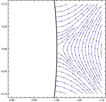
The story goes like this. A paper was published in Nature giving a measurement of the mass of the black hole in question. (Full article access from Nature is paywalled. Here’s the free Arxiv version, which appears to be substantively identical.) The key figure:

According to Gould, “The contours of Figure 2 of Davis et al. (2013) reflect χ²/dof.” That last bit is “chi-squared per degree of freedom,” also known as “reduced chi-squared.” If that’s true, then the authors have definitely made a mistake. The recipe described in the figure caption for turning chi-squared contours into error estimates is based on (non-reduced) chi-squared, not chi-squared per degree of freedom.

The Davis et al. paper doesn’t clearly state that Figure 2 shows reduced chi-squared, and Gould doesn’t say how he knows that it does, but comments in Peter Coles’s blog, which is where I first heard about this paper, seem to present a convincing case that Gould’s interpretation is right. See in particular this comment from Daniel Mortlock, which says in part

Since posting my comment above I have exchanged e-mails with Davis and Gould. Both confirm that the contours in Figure 2 of Davis et al. are in fact chi^2/red or chi^2/dof, so the caption is wrong and Gould’s re-evaluation of the uncertainty in M_BH is correct . . .

. . . at least formally. The reason for the caveat is that, according to Davis, there are strong correlations between the data-points, so the constraints implied by ignoring them (as both Davis and Gould have done so far) are clearly too tight.

So it appears that Gould correctly identified an error in the original analysis, but both papers cheerfully ignore another error that could easily be extremely large! Ignoring “strong correlations” when calculating chi-squareds is not OK.

So this is quite a messy story, but the conclusion seems to be that you shouldn’t have much confidence in either error estimate.

I find myself wondering about the backstory behind Gould’s paper. When you find an error like this in someone else’s work, the normal first step is to email the authors directly and give them a chance to sort it out. I wonder if Gould did this, and if so what happened next. As we all know, people are reluctant to admit mistakes, but the fact that reduced chi-squared is the wrong thing to use here is easily verified. (I guarantee you that at least some of the authors have a copy of the venerable book Numerical Recipes on their shelves, which has a very clear treatment of this.) Moreover, the error in question makes the authors’ results much stronger and more interesting (by reducing the size of the error bar), which should make it easier to persuade them.

The other strange thing in Gould’s paper is the last phrase of the abstract: “an error that I suggest may be common among astronomers.” His evidence for this is that he saw one other paper recently (which he doesn’t cite) that contained the same error. Coming from someone who’s clearly concerned about correctly drawing inferences from data, this seems like weak evidence.

One last thing. Peter Coles’s post drawing attention to this paper casts it as a Bayesian-frequentist thing:

The “mathematical error” quoted in the abstract involves using chi-squared-per-degree-of-freedom instead of chi-squared instead of the full likelihood function instead of the proper, Bayesian, posterior probability. The best way to avoid such confusion is to do things properly in the first place. That way you can also fold in errors on the distance to the black hole, etc etc…

At first, I have to admit that I wasn’t sure whether he was joking here or not. Sometimes I have trouble recognizing that understated, dry British sense of humor. (I guess that’s why I never fully appreciated Benny Hill.)

Anyway, this isn’t about the whole Bayesian-frequentist business. The various errors involved here (using reduced chi-squared and ignoring correlations) are incorrect from either point of view. Suppose someone put a batch of cookies in a gas oven, forgot about them, and came back two hours later to find them burnt. You wouldn’t say, “See? That’s why electric ovens are much better than gas ovens.”

Peter’s riposte:

The problem is that chi-squared is used by too many people who don’t know (or care) what it is they’re actually trying to do. Set it up as a Bayesian exercise and you won’t be tempted to use an inappropriate recipe.

Or set it up as a frequentist exercise and you’ll do it right too, as long as you think clearly about what you’re doing. This is an argument against doing things without thinking about them carefully, nothing more.

As long as I’ve come this far, in case anyone’s wondering, here’s my position, to the extent I have one, on the Bayesian-frequentist business:

• The frequentist interpretation of the meaning of probabilities is incoherent.
• It’s perfectly OK to use frequentist statistical techniques, as long as you know what you’re doing and what the results of such an analysis mean. In particular, a frequentist analysis never tells you anything about the probability that a theory is true, just about the probability that, if a theory is true, the data that you see would occur.
• As a corollary of the last point, even if you’ve used frequentist techniques to analyze your data, when you want to draw conclusions about the probabilities that various theories are true, you have to use Bayesian inference. There’s simply no other coherent way to do this sort of reasoning. Even frequentists do this, although they may not admit it, even to themselves.
• Given that you have to use Bayesian inference anyway, it’s better to be open about it.

I’m a bit slow getting to this: Sean Carroll, Matt Strassler, and probably others wrote about it days ago. But I’m still irritated about it, so I’ll go ahead.

CBS News says this about the Higgs boson:

The Higgs boson is often called “the God particle” because it’s said to be what caused the “Big Bang” that created our universe many years ago.

This is wrong. There is absolutely no sense in which the Higgs caused the Big Bang.

Just to be clear, this is not a case of oversimplifying or leaving out some technical provisos. It’s just completely wrong. It’s about as accurate as the following:

The Higgs boson is the key to making a delicious flaky pie crust.

Actually, that analogy’s not really fair: the Higgs has far more to do with making a pie crust than it does with causing the Big Bang. After all, there’s chemistry involved in making the pie crust. Chemistry depends on the mass of the electron, which (unlike the Big Bang) crucially depends on the Higgs.

It’s not too surprising for a news outlet to make this mistake. You might be tempted to say that physicists brought it on ourselves by stupidly calling the damn thing the God particle. In general, there’s some truth to this accusation, but in this instance, physicists (plural) aren’t to blame — one physicist is. CBS was directly quoting famous science popularizer Michio Kaku.

CBS got this wrong, which is forgivable. Kaku, on the other hand, lied about it, which is much worse. That is, the person who wrote the CBS article presumably and reasonably believed that the statement was true. Kaku certainly knew it was false when he said it. Whatever one may think of him as a science popularizer, there’s no doubt that he’s a competent particle physicist, and no competent particle physicist would believe that statement.

Kaku has a history of exaggerating and embellishing when he talks about science. I understand the desire to simplify when explaining things to a general audience, but there’s a big difference between simplifying and lying. Every time a scientist does this, he erodes the credibility of all scientists just a little bit.

Strassler’s blog post is aptly titled Why, Professor Kaku? Why? Not having access to the inside of Kaku’s brain, I don’t know, but it seems to me the most plausible guess is the following:

• Kaku wanted to convey the idea that the Higgs is exciting (which is true).
• It’s hard to explain why the Higgs is exciting (also true).
• Everyone knows the Big Bang is exciting (definitely true).
• So he decided to convey the excitement by linking the Higgs to the Big Bang.

Personally, I think flaky pie crust is quite exciting, so I think he should have gone with that.

Jerry Coyne stumbled on the following, from Paul Davies:

Q: Do you think one reason the multiverse theory has become so popular in recent years is to keep the whole idea of God at bay?

A [Davies]: Yes.

Then later

“There’s no doubt that the popularity of the multiverse is due to the fact that it superficially gives a ready explanation for why the universe is bio-friendly. Twenty years ago, people didn’t want to talk about this fine-tuning because they were embarrassed. It looked like the hand of a creator. Then along came the possibility of a multiverse, and suddenly they’re happy to talk about it because it looks like there’s a ready explanation. . . Even the scientific explanations for the universe are rooted in a particular type of theological thinking. They’re trying to explain the world by appealing to something outside of it.”

In case you don’t have your scorecard handy, Coyne is a scientist with a very strong skeptical stance. Davies is a physicist who is Christian and generally “accommodationist” — that is, he tends to argue in favor of the compatibility of science and religion. [Update: Apparently I was wrong to describe Davies as Christian — see comments below. My apologies for the error.]

Coyne rightly detects the scent of bullshit here. Physicists these days talk quite a bit about theories involving multiple universes, for reasons that come out of various scientific arguments, not for anti-religious reasons at all. If you want to know more, and you’re going to be a first-year student at UR next year, take my first-year seminar, Space is Big. If you’re not, you could do a lot worse than to read Brian Greene’s book on the subject.

Coyne quotes Sean Carroll extensively to explain why Davies is wrong. From Coyne’s blog post:

The multiverse idea isn’t a “theory” at all; it’s a prediction made by other theories, which became popular for other reasons. The modern cosmological version of the multiverse theory took off in the 1980′s, when physicists took seriously the fact that inflationary cosmology (invented to help explain the flatness and smoothness of the early universe, nothing to do with God) often leads to the creation of a multiverse (see here for a summary). It gained in popularity starting around the year 2000, when string theorists realized that their theory naturally predicts a very large number of possible vacuum states (see e.g. http://arxiv.org/abs/hep-th/0302219). All along, cosmologists have been trying to take the predictions of their models seriously, like good scientists, not trying to keep God at bay.

This is all exactly right. But one thing Carroll and Coyne don’t point out is that Davies is wrong in his premise, not just his conclusion. To be specific, this is quite simply factually false:

Twenty years ago, people didn’t want to talk about this fine-tuning because they were embarrassed.

I happen to have been hanging around one of the leading cosmology groups in the world at that time (as a graduate student at UC Berkeley), and I can tell you that everyone talked about fine-tuning all the time.

At that time, multiverse-based explanations were not popular, and the various fine-tuning problems (i.e., why conditions in the Universe seemed to be surprisingly well-adapted for life) were regarded as mysterious and as-yet unsolved problems. Davies would have you believe that we didn’t want to talk about those problems because we didn’t have good (non-religious) answers to them. On the contrary, because we didn’t have answers to them, we talked about them incessantly. That’s what scientists do: there’s nothing we like more than a meaty unsolved problem! The idea that we were afraid of this sort of problem because it might force us into dangerous religious territory is the precise opposite of the truth.

Cosmologists have been waiting a long time for the release of the Planck satellite’s cosmic microwave background data. The wait is over:

 

 

 

 

The Planck data has finer resolution (i.e., can see sharper details) than the previous all-sky WMAP data, as illustrated in this picture (which, like the previous one, is from the European Space Agency, which runs Planck):

 

There are other important differences. Both data sets are made from maps at multiple different frequencies, but Planck’s frequencies cover a wider range. This is nice, because it makes it possible to separate out the different constituents of the map more precisely. To be specific, the raw data include both the cosmic microwave background radiation and other, more local “foregrounds,” such as emission from stuff in our own Galaxy. The pictures above show just the CMB component.

Along with the data, the Planck collaboration released 29 papers‘ worth of analysis, which have been submitted for publication but have not yet undergone peer review. Obviously, people will be digesting all this information, and using the data for their own studies, for a long time.

As far as I can tell, there are no huge surprises. The most important scientific product you get from a data set like this is the power spectrum, which looks like this:

The red points are the measurements, which match the theoretical prediction very well. You can estimate various parameters from this fit, including the amount of dark matter (somewhat bigger than previously thought) and the expansion rate of the Universe (a bit slower than previously thought).

The value of the parameter known as the spectral index n is of interest to specialists, although not to anyone else: it’s about 0.96 plus or minus 0.01. The main point is that it’s significantly different from 1. Here’s what that means: if you take the variations in density in the early Universe, and model them as a sum of sine waves of different wavelengths, the long-wavelength waves are slightly more important than the short-wavelength waves. n=1 would have corresponded to all wavelengths being equally important. If you’re not in the business, you probably still don’t care, and that’s OK, but it’s interesting to some people (basically because some theoretical models predict this and others don’t).

Finally, there’s the fact that the so-called “large-scale anomalies” in the maps didn’t go away. These are patterns or features that showed up in the earlier WMAP data but were not expected by our best theories:

• The level of fluctuations on very large angular scales is smaller than expected.
• One half of the sky has slightly smaller temperature variations than the other.
• The largest-scale multipoles (i.e., the longest-wavelength waves you get if you model the data as a combination of ripples of different wavelengths) tend to line up in a certain direction, whereas our theories say the directions should be random.

People argue over how much (if any) interest we should take in the anomalies. Before Planck, you could reasonably adopt any of the following stances:

1. The anomalies are a result of some sort of problem in the data processing.
2. The anomalies are due to some sort of foreground contaminant (i.e., local stuff, not stuff from the early Universe).
3. The anomalies are present in the CMB, but they’re just chance fluctuations without any greater significance.
4. The anomalies are telling us something new and important about the Universe.

At a quick glance, the Planck data make it much harder to believe the first two. The differences between the two data sets are such that you wouldn’t expect the anomalies to look similar if they were processing artifacts or foregrounds, but they do look similar. Both 3 and 4 are still viable.

It’s hard to decide between 3 and 4. You might think that you could assess the validity of #3 by the  usual methods of calculating statistical significances. The problem is that the anomalies were noticed in the data first, and their level of improbability was only calculated after the fact. That means that you can’t calculate statistical significances in a meaningful way. In any large data set, there are so many things you could choose to look at that you’re bound to find some that are unlikely. Maybe that’s all the CMB anomalies are. (Here’s a perhaps slightly labored analogy with the Super Bowl coin toss.)

Personally, I don’t know whether the CMB anomalies are telling us anything, but I’m glad they’re still around. I have a bit of a soft spot for them.

 

That’s an old principle, often attributed to David Hume if I’m not mistaken. It means that there’s no chain of reasoning that takes you from factual statements about the way the world is to normative statements about the way things should be.

That’s not to say that factual statements are irrelevant to ethical questions, just that when you’re engaged in ethical reasoning you need some sort of additional inputs.

Religious traditions often give such inputs. For the non-religious, one common point of view is utilitarianism, which is the idea that you ought to do the things that will maximize some sort of total worldwide “utility” (or “happiness” or “well-being” or something like that). The point is that in either case you have to take some sort of normative (“ought”) statement as an axiom, which can’t be derived from observations about the way the world is.

For what it’s worth, I think that Hume is right about this.

The reason I’m mentioning all this utterly unoriginal stuff right now is because I want to link to a piece that Sean Carroll wrote on all this. In my opinion, he gets it exactly right.

Sean’s motivation for writing this is that some people claim from time to time that ethics can be (either now or in the future) reduced to science — i.e., that we’ll be able to answer questions about what ought to be done purely by gathering empirical data. Sam Harris is probably the most prominent proponent of this point of view these days. If Hume (and Sean and I) are right, then this can’t be done without additional assumptions, and we need to think carefully about what those assumptions are and whether they’re right.

I haven’t read Harris’s book, but I’ve read some shorter pieces he’s written on the subject. As far as I can tell (and I could be wrong about this), Harris seems to take some sort of utilitarianism for granted — that is, he takes it as self-evident that (a) there is some sort of global utility that (at least in principle) can be measured, and that (b) maximizing it is what one ought to do.

Personally, I don’t think either of those statements is obvious. At the very least, they need to be stated explicitly and supported by some sort of argument.

 

I recently mentioned a couple of new things I’d learned in teaching an electricity and magnetism class this semester. One is the answer to this question:

Charge Q is placed on an infinitely thin conducting disk of radius R. How does it distribute itself over the disk?

 The answer turns out to be that the charge distribution is the same as if you started with a uniform distribution of charge over a spherical shell, and compressed the shell down to a disk by smashing each piece of the surface straight up or down in the direction perpendicular to the disk.

Although I know of various proofs of this, particularly one provided by my friend and colleague Ovidiu Lipan, none of them seemed to me like a satisfying explanation of why the result was true. Of course, there might not be such a thing, but when the final answer has such a simple description (compared to most problems in E&M, which have incredibly messy solutions), it seems like there ought to be a nice reason for it.

Later I came across some notes by Kirk McDonald of Princeton provide a somewhat intuitive answer. I’ll summarize the idea here.

Start with something every E&M student should know. Take a spherical shell of radius R and thickness dR, and fill it uniformly with charge. Then the electric field inside the shell is zero. The slick way to prove this is with Gauss’s Law, but you can prove it with more basic geometric reasoning as follows. (In fact, I believe that the argument goes all the way back to Newton, although of course he wasn’t talking about electric fields, since they hadn’t been discovered / invented yet).

Say that you’re located at an arbitrary point inside the spherical shell. Draw two cones with infinitesimal solid angle going out in opposite directions. These intersect the shell giving two little “charge elements” shown in red below.

You can convince yourself that the electric field contributions from these charge elements exactly cancel each other. The volume, and hence the amount of charge, of each is proportional to the square of its distance from you, so by the inverse square law they give equal but opposite fields.

Since you can chop up the whole shell into such pairs, the total electric field vanishes.

The clever insight in McDonald’s notes is that the same argument holds even if you take the spherical shell and compress it into an ellipsoid (i.e., rescale all of the z coordinates by some constant factor, while leaving x and y the same):

With a bit of effort, you can convince yourself that all the various distances and volumes scale in such a way that the two field contributions remain equal and opposite.

Now that we know that the field inside this ellipsoid is zero, what can we conclude? First, take the limit as dR goes to zero, so we have a two-dimensional surface charge distribution. The result must be the same as the surface charge distribution on a solid, conducting ellipsoid. After all, the conducting ellipsoid has to have charge only on its surface and have zero field inside. The usual electrostatic uniqueness theorems apply here, which say that there’s only one charge distribution that leads to this result. Since we’ve found a charge distribution that does so, it must be the charge distribution.

Keep smashing the ellipsoid down until it lies in a plane, and you’ve got the solution for the conducting disk.

An appeals court in England has apparently ruled that Bayesian reasoning (also known as “correct reasoning”) about probability is invalid in the British court system.

The case was a civil dispute about the cause of a fire, and concerned an appeal against a decision in the High Court by Judge Edwards-Stuart. Edwards-Stuart had essentially concluded that the fire had been started by a discarded cigarette, even though this seemed an unlikely event in itself, because the other two explanations were even more implausible. The Court of Appeal rejected this approach although still supported the overall judgement and disallowed the appeal.

I learned about this from Peter Coles’s blog, which also mentions a similar ruling in a previous case.

From the judge’s ruling (via understandinguncertainty.org):

When judging whether a case for believing that an event was caused in a particular way is stronger that the case for not so believing, the process is not scientific (although it may obviously include evaluation of scientific evidence) and to express the probability of some event having happened in percentage terms is illusory.

The judge is essentially saying that Bayesian inference is unscientific, which is the exact opposite of the truth. The hallmark of science is the systematic use of evidence to update one’s degree of belief in various hypotheses. The only way to talk about that coherently is in the language of probability theory, and specifically in the language of Bayesian inference.

Apparently the judge believes that you’re only allowed to talk about probabilities for events that haven’t happened yet:

The chances of something happening in the future may be expressed in terms of percentage. Epidemiological evidence may enable doctors to say that on average smokers increase their risk of lung cancer by X%. But you cannot properly say that there is a 25 per cent chance that something has happened. Either it has or it has not.

The author of that blog post gives a good example of why this is nonsense:

So according to this judgement, it would apparently not be reasonable in a court to talk about the probability of Kate and William’s baby being a girl, since that is already decided as true or false.

Anyone who has ever played a card game should understand this. When I decide whether to bid a slam in a bridge game, or whether to fold in a poker game, or whether to take another card in blackjack, I do so on the basis of probabilities about what the other players have in their hands. The fact that the cards have already been dealt certainly doesn’t invalidate that reasoning.

I’m a mediocre bridge player and a lousy poker player, but I’d love to play with anyone who I thought would genuinely refuse to base their play on probabilistic reasoning.

Probabilities give a way, or rather the way, to talk precisely about degrees of knowledge in situations where information is incomplete. It doesn’t matter if the information is incomplete because some event hasn’t happened yet, or simply because I don’t know all about it.

By the way, Peter Coles makes a point that’s worth repeating about all this. Statisticians divide up into “Bayesian” and “frequentist” camps, but this sort of thing actually has very little to do with that schism:

First thing to say is that this is really not an issue relating to the Bayesian versus frequentist debate at all. It’s about a straightforward application of Bayes’ theorem which, as its name suggests, is a theorem; actually it’s just a straightforward consequence of the sum and product laws of the calculus of probabilities. No-one, not even the most die-hard frequentist, would argue that Bayes’ theorem is false.

Even if you’re a benighted frequentist in matters of statistical methodology, the way you think about probabilities still involves Bayes’s theorem.

I’m teaching our course in Electricity and Magnetism this semester, and even though I’ve done this plenty of times before, I still learn new things each time. Here are a couple from this semester.

1. Charged conducting disk.

Suppose I take a thin disk of radius R, made out of a conducting material, and put a given amount of charge Q on it. How does the charge distribute itself?  (In case it’s not clear, the disk lives in three-dimensional space but has negligible thickness. In other words, it’s a cylinder of radius R and height h, in the limit h << R.)

This turns out to have a surprisingly simple answer. Take a sphere of radius R, and distribute the charge uniformly over the surface. Now smash the sphere down to a disk by moving each element of surface area straight down parallel to the z axis. The resulting charge density is the answer.

My friend and colleague Ovidiu Lipan showed me a proof of this, and then I verified it numerically using Mathematica, so I’m confident it’s right. But I still have the feeling there’s more to the story than this. This result is simple enough that it seems like there should be a satisfying, intuitive reason why it’s true. Although Ovidiu’s proof is quite clever and elegant, it doesn’t give me the feeling that I understand why the result came out in this neat way. I’d love to hear any ideas.

Update: These notes by Kirk McDonald have the answer I was looking for. I’ll try to write a more detailed explanation at some point.

2. Electric field lines near a conducting sphere.

Take a conducting sphere and place it in a uniform external electric field. Find the resulting potential and electric field everywhere outside the sphere.

This is a classic problem in electrostatics. I’ve assigned it plenty of times before, but I learned a little something new about it, once again from the exceedingly clever Ovidiu Lipan (who apparently got it from an old book by Sommerfeld).

You can calculate the answer using standard techniques (separation of variables in spherical coordinates). The external field induces negative charge on the bottom of the sphere and positive charge on the top, distorting the field lines until they look like this:

 

This picture looks just as you’d expect. In particular, one of the first things you learn about electrostatics is that field lines must strike the surface of a conductor perpendicular to the surface.

Let’s zoom in on the region near the sphere’s equator:

The field lines either strike the southern hemisphere, emanate from the northern hemisphere, or miss the sphere entirely. All is as it should be.

Or is it? Let me put in a couple of additional field lines:

 

The curves in red are legitimate electric field lines (i.e., the electric field at each point is exactly tangent to the curve), but they don’t hit the surface at a right angle as they’re supposed to. You can actually write down an exact equation for these lines and verify that they come it at 45-degree angles right up to the edge of the sphere.

We constantly repeat to our students that electric field lines have to hit conductors at right angles. So is this a lie?

Ultimately, it’s a matter of semantics. You can say if you want that those red field lines don’t actually make it to the surface: right at the sphere’s equator, the electric field drops to zero, so you could legitimately say that the field line extends all the way along an open interval leading up to the sphere’s edge, but doesn’t include that end point. This means you have to allow an exception to another familiar rule: electric field lines always start at positive charges and end at negative charges (unless they go to infinity). Here we have field lines that just peter out at a place where the charge density is zero.

Alternatively, you can say that there’s an exception to the rule that says electric field lines have to hit conductors at right angles: they have to do this only if the field is nonzero at the point of contact. After all, the “must-hit-perpendicular” is really a rephrasing of the rule that says that the tangential component of the electric field must be zero at a conductor. The latter version is still true, but it implies the former version only if the perpendicular component is nonzero.

People sometimes ask me whether, as a scientist, I get annoyed by scientific inaccuracies in movies. Sometimes, I guess, but not usually. In science fiction, I think it’s fine if the fictional world you’ve created breaks the rules of our actual universe, as long as it consistently follows its own rules.

I actually find  linguistic inaccuracies in historical fiction more annoying than scientific inaccuracies in science fiction. For some reason, linguistic anachronisms raise my nerd hackles.

I was thinking about this recently because, as a middle-aged Prius-driving NPR listener, I am legally obliged to watch Downton Abbey. 

Twice during the current season, characters have described themselves as being “on a learning curve,” in one case “on a steep learning curve.” This phrase is irritating enough in contemporary parlance, but in the mouths of 1920s characters it’s all the more grating.

I posted a gripe about it on Facebook, with some actual data from the awesome Google Ngram viewer:

A friend made the fair observation that “learning curve” goes back further than “steep learning curve”:

If Matthew Crawley and Tom Branson were linguistic trendsetters, maybe they could have been saying this in the 1920s, but I’m not buying it, and Ngram will help me justify my skepticism. I knew Ngram had an amazingly huge corpus of searchable books, but it turns out to be more powerful and flexible than I’d realized.

I suspect that the term was only used in a technical context, to describe actual graphs of learning, until much, much later. The citations of the phrase in the OED are consistent with this, but there are only a couple of them, so that’s not much evidence. Ngram can help with this: we can look at the phrase’s popularity in just fiction, rather than in all books.

The phrase takes off in fiction in the last couple of decades, around when (I claim) people actually started saying it in non-technical contexts. Also, in the early years, it was almost entirely an American phrase:

 

(That’s all books, not just fiction.)

Another Downton linguistic anachronism: “contact” as a verb. I’d originally searched Ngram for “contacted” to illustrate this, but it turns out that you can tell it to search for words used as particular parts of speech. Here’s “contact” as both verb and noun:

(Verb in blue, amplified by a factor of 10 for ease of viewing.)

The fact that you can do this strikes me as quite impressive technically. Not only have they scanned in all these books and converted them to searchable text, but they’ve parsed the sentences to identify all the parts of speech. That’s a nontrivial undertaking. As Groucho Marx apparently never said, “Time flies like an arrow; fruit flies like a banana.”

The phrase “have a crush on” also came up and sounded off to me, but I was pretty much wrong on that. It was starting to become common in the 1920s, although it was mostly American:

In hindsight, I should have known that: the Gershwin song “I’ve got a crush on you” dates from a bit later than Downton, but not that much.

Funny thing about living in a smallish city: I’m the only astrophysicist in town, so the news media sometimes ask me about space stories in the news. Here’s the latest.

Richmond’s Channel 8 talked to me about the Russian meteor. Video here and here.

I’m annoyed that I seem to have said this event was similar in size to Tunguska, when in fact it was much smaller. But I was doing this on virtually no preparation, so I guess it could have been worse.